Introducing the Hamilton library

Hamilton: README / hackage / github

The hamilton library is on hackage! It was mostly a proof-of-concept toy experiment to simulate motion on bezier curves, but it became usable enough and accurate enough (to my surprise, admittedly) that I finished up some final touches to make it complete and put it on hackage as a general-purpose physics simulator.

The library is, in short, a way to simulate a physical system by stating nothing more than an arbitrary parameterization of a system (a “generalized coordinate”) and a potential energy function.

I was going to write a Haskell post on the implementation, which was what interested me at first. I wanted to go over –

1. Using automatic differentiation to automatically compute momentum and the hamilton equations, which are solutions of differential equations.

2. Using type-indexed vectors and dependent types in a seamless way to encode the dimensionality of the generalized coordinate systems and to encode invariants the types of functions.

And fun stuff like that. But that post might be a bit of a while away, so I’m just going to write a post about the usage of the library. (Fair warning, most of this information is also found in the readme.)

Hamiltonian Mechanics

(This section goes briefly over some relevant part of the physics behind Hamiltonian dynamics, but feel free to skip it if you want to go straight to the Haskell)

Hamiltonian mechanics is a brilliant, radical, and beautiful re-imagination of the physics of mechanics and dynamics by William Rowan Hamilton. It was adapted for statistical mechanics and thermodynamics, and it was through the lens of Hamiltonian mechanics that Schroedinger and Heisenberg independently found insight that unlocked the secrets of quantum mechanics. While Newton’s interpretation of mechanics (in terms of forces and accelerations) was cute, it simply didn’t generalize to quantum mechanics. Hamiltonian’s interpretation of mechanics did, and we have a century of physics revolutions to thank for it. Hamiltonian mechanics also generalize without any extra work to relativity – another case where newtonian mechanics tends to fall apart.

Hamiltonian mechanics, in a classical sense, imagines that the state of the system exists as a point in phase space, and that the system evolves based on geometric properties of the system’s Hamiltonian over that phase space.

In other words, define the Hamiltonian of the system, and you see the step-by-step evolution and dynamics of the system. You can imagine mechanics as a series of streams of flow over phase space…and the state of the system just goes along for the ride.

One nice thing about phase space is that it can be stated in terms of any arbitrary parameterization/coordinate system of your system. For example, for a double pendulum system, you can imagine the system as traveling about in the phase space of the angles of the bobs (instead of their actual positions in cartesian space). If you can find any way to parameterize your system, in any sort of type of coordinates, then Hamiltonian mechanics will describe how it evolves in those coordinates.

State some fundamental geometric properties about your coordinate system, and the Hamiltonian figures out the rest. It’s the key to unlocking the dynamical properties of the system.

I could go into more details, but this isn’t a post about Hamiltonian mechanics! Armed with this, let’s look into modeling an actual double pendulum system in terms of the angles of the bobs.

Examples

The Double Pendulum

So, if we’re going to be simulating a double pendulum system using hamilton, we need three things:

1. A statement of our parameterized coordinates and how they relate to the underlying cartesian coordinates of our system

2. The inertias (in our case, masses) of each of those underlying coordinates.

3. A potential energy function (in our case, just the potential energy induced by gravity)

We have two coordinates here (\(\theta_1\) and \(\theta_2\)), which will be encoding the positions of the two pendulums:

\[ \langle x_1, y_1 \rangle = \left\langle \sin (\theta_1), - \cos (\theta_1) \right\rangle \]

\[ \langle x_2, y_2 \rangle = \left\langle \sin (\theta_1) + \frac{1}{2} \sin (\theta_2), - \cos (\theta_1) - \frac{1}{2} \cos (\theta_2) \right\rangle \]

(Assuming that the first pendulum has length 1 and the second pendulum has length \(\frac{1}{2}\))

The inertias of \(x_1\), \(y_1\), \(x_2\), and \(y_2\) are the “masses” attached to them. Let’s pick that the first bob has mass \(1\) and the second bob has mass \(2\), so then our masses are \(\langle 1, 1, 2, 2 \rangle\).

Finally, the potential energy of our system is just the potential energy of gravity, \(m \times g \times y\) for each of our points:

\[ U(x_1, y_1, x_2, y_2) = ( y_1 + 2 y_2 ) g \]

Turns out that this is a complete enough description of our system to let hamilton do the rest!

-- source: https://github.com/mstksg/inCode/tree/master/code-samples/hamilton/DoublePendulum.hs#L10-L25

doublePendulum :: System 4 2
doublePendulum = mkSystem' masses coordinates potential
  where
    masses :: R 4
    masses = vec4 1 1 2 2
    coordinates
        :: Floating a
        => V.Vector 2 a
        -> V.Vector 4 a
    coordinates (V2 θ1 θ2) = V4 (sin θ1)            (-cos θ1)
                                (sin θ1 + sin θ2/2) (-cos θ1 - cos θ2/2)
    potential
        :: Num a
        => V.Vector 4 a
        -> a
    potential (V4 _ y1 _ y2) = (y1 + 2 * y2) * 5    -- assuming g = 5

(with some helper patterns defined here – V2 and V4 – that lets us pattern match on and construct sized Vectors and their 2 (or 4) elements)

Ta dah. That’s literally all we need.

A System m n represents a description of a physical system (without its state) described with n parameters/generalized coordinates. The m represents the dimension of its underlying cartesian coordinate system (4 for us, with \(\langle x_1, y_1, x_2, y_2 \rangle\)). The m should be more or less irrelevant to the actual usage of System m n and the hamilton api…but it’s mostly useful only if we eventually want to plot the system in normal cartesian space.

Now, let’s run the simulation. First we have to pick a starting configuration:

-- source: https://github.com/mstksg/inCode/tree/master/code-samples/hamilton/DoublePendulum.hs#L37-L39

config0 :: Config 2
config0 = Cfg (vec2 1 0  )  -- initial positions
              (vec2 0 0.5)  -- initial velocities

A Config n represents the state of the system, represented in configuration-space. But, remember, Hamiltonian dynamics is about simulating the path of the particle through phase space. So we can convert our configuration-space state into a phase-space state:

-- source: https://github.com/mstksg/inCode/tree/master/code-samples/hamilton/DoublePendulum.hs#L41-L42

phase0 :: Phase 2
phase0 = toPhase doublePendulum config0

And now we can ask for the state of our system at any amount of points in time:

-- source: https://github.com/mstksg/inCode/tree/master/code-samples/hamilton/DoublePendulum.hs#L44-L45

evolution :: [Phase 2]
evolution = evolveHam' doublePendulum phase0 [0,0.1 .. 1]

The result there will be the state of the system at times 0, 0.01, 0.02, 0.03 … etc.

Or, if you want to run the system step-by-step:

-- source: https://github.com/mstksg/inCode/tree/master/code-samples/hamilton/DoublePendulum.hs#L47-L48

evolution' :: [Phase 2]
evolution' = iterate (stepHam 0.1 doublePendulum) phase0

And you can get the position of the coordinates as:

-- source: https://github.com/mstksg/inCode/tree/master/code-samples/hamilton/DoublePendulum.hs#L50-L51

positions :: [R 2]
positions = phsPositions <$> evolution'

With phsPositions :: Phase n -> R n

And the position in the underlying cartesian space as:

-- source: https://github.com/mstksg/inCode/tree/master/code-samples/hamilton/DoublePendulum.hs#L53-L54

positions' :: [R 4]
positions' = underlyingPos doublePendulum <$> positions

Where underlyingPos :: System m n -> Phase n -> R m.

Let’s ignore the underlying position for now, and print out now the full progression of the system’s positions:

-- source: https://github.com/mstksg/inCode/tree/master/code-samples/hamilton/DoublePendulum.hs#L56-L57

main :: IO ()
main = withRows (take 25 positions) (disp 4)

(withRows is from hmatrix, which treats a list of vectors as a matrix with each vector as a row, and disp 5 from hmatrix pretty-prints our matrix with 5 decimal places of precision)

L 25 2
 1.0000   0.0000
 0.9727   0.0800
 0.8848   0.2345
 0.7164   0.5129
 0.4849   0.8725
 0.2878   1.0648
 0.1223   1.0801
-0.0165   0.9388
-0.1099   0.6400
-0.1161   0.1447
-0.0539  -0.4882
-0.0795  -0.9212
-0.1689  -1.1797
-0.2860  -1.2970
-0.4146  -1.2803
-0.5562  -1.1238
-0.7249  -0.8079
-0.8762  -0.4505
-0.9442  -0.2075
-0.9416  -0.0516
-0.8793   0.0312
-0.7596   0.0265
-0.5728  -0.1086
-0.3001  -0.4237
-0.0381  -0.6640

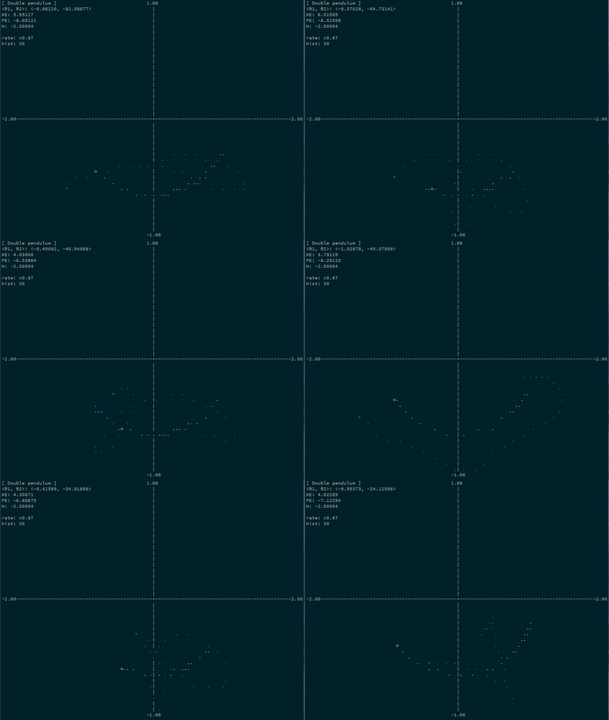
Neat! We see that the first coordinate (\(\theta_1\)) starts at 1 like we asked, and then begins decreasing and falling… And then we see the second coordinate (\(\theta_2\)) starting at 0 and then “swinging” to the right. The image the top of this post is an animation of such a system (albeit with \(m_2 = 1\)).

Two-body system

Here’s one more situation where generalized coordinates describe things in a lot nicer way than cartesian coordinates: the classic two-body problem.

Really, you can describe the state of a two-body system with only two parameters: the distance between the two bodies, and their current angle of rotation.

In this framework, Kepler tells us that for bodies in orbit, the distance will grow smaller and larger again over time, and that the angle of rotation will constantly increase…and increase at a faster rate when the distance is smaller (which is Kepler’s second law).

If we assume that the center of mass of the system is at \(\langle 0, 0 \rangle\), then we can state these coordinates as

\[ \langle x_1, y_1 \rangle = \langle r_1 \cos (\theta), r_1 \sin (\theta) \rangle \]

\[ \langle x_2, y_2 \rangle = \langle r_2 \cos (\theta), r_2 \sin (\theta) \rangle \]

Where \(r_1 = \frac{m_2}{m_1 + m_2}\) and \(r_2 = - \frac{m_1}{m_1 + m_2}\) (solving from the center of mass).¹

Our potential energy function is Newton’s famous law of universal gravitation:

\[ U(r, \theta) = - \frac{G m_1 m_2}{r} \]

And, this should be enough to go for hamilton.

“But wait,” I hear you say. “If we’re doing a change-of-coordinate-system into polar coordinates, don’t we have to account for artifacts like centrifugal acceleration from the fact that \(d \theta\) is non-uniform and depends on \(r\)?”

Well, I’m glad you asked! And the answer is, nope. We don’t have to account for any weird interplay from non-uniform coordinate systems because hamilton arrives at the proper solution simply from the geometry of the generalized coordinates. (And it does this using ad, but more on that for a later post!)

Anyway, here we go:

-- source: https://github.com/mstksg/inCode/tree/master/code-samples/hamilton/TwoBody.hs#L10-L42

twoBody :: System 4 2
twoBody = mkSystem masses coordinates potential
  where
    masses :: R 4
    masses = vec4 10 10 1 1
    coordinates
        :: Floating a
        => V.Vector 2 a
        -> V.Vector 4 a
    coordinates (V2 r θ) = V4 (r1 * cos θ) (r1 * sin θ)
                              (r2 * cos θ) (r2 * sin θ)
      where
        r1 =   r *  1 / 11
        r2 = - r * 10 / 11
    potential
        :: Fractional a
        => V.Vector 2 a
        -> a
    potential (V2 r _) = - 10 / r       -- G = 1

config0 :: Config 2
config0 = Cfg (vec2 2   0)  -- initial positions
              (vec2 0 0.5)  -- initial velocities

(we use mkSystem instead of mkSystem' because we want to state the potential energy in terms of our generalized coordinates \(r\) and \(\theta\))

Let’s take a peek:

-- source: https://github.com/mstksg/inCode/tree/master/code-samples/hamilton/TwoBody.hs#L44-L60

phase0 :: Phase 2
phase0 = toPhase twoBody config0

evolution' :: [Phase 2]
evolution' = iterate (stepHam 0.1 twoBody) phase0

positions :: [R 2]
positions = phsPositions <$> evolution'

main :: IO ()
main = withRows (take 25 positions) (disp 4)

L 25 2
2.0000  0.0000
1.9887  0.0502
1.9547  0.1015
1.8972  0.1554
1.8149  0.2133
1.7058  0.2777
1.5669  0.3523
1.3933  0.4435
1.1774  0.5647
0.9057  0.7503
0.5516  1.1413
0.2057  3.4946
0.6092  5.2275
0.9490  5.5664
1.2115  5.7386
1.4207  5.8542
1.5889  5.9424
1.7233  6.0152
1.8283  6.0785
1.9069  6.1358
1.9610  6.1892
1.9917  6.2403
1.9998  6.2904
1.9852  6.3407
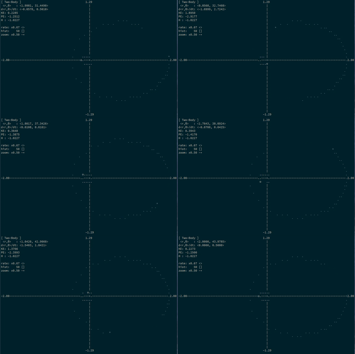
1.9479  6.3923

Neat! We see that \(r\) starts big and gets smaller, and then gets big again. And it’s clear that when \(r\) is smallest, \(\theta\) changes the fastest. Look at it go!

Here’s an animation of the same situation with some different masses:

Just you wait

Now, this isn’t all just useful for physics. You can state a lot of animation/dynamics problems as motion along coordinates that aren’t always trivial. This project started, after all, as a way to simulate constant-velocity motion along a bezier curve. (In that case, the single coordinate is the non-uniform time parameter to the bezier curve.)

I’ve included more examples in the example app launcher included in the library (which generated those animations you see above), including:

1. A spring hanging from a block sliding along a horizontal rail (a favorite of many physics students, of course)
2. A ball bouncing around a room, showing that you can represent bouncy walls as potential energy functions
3. The bezier curve example.

Let me know in the comments if you think of any interesting systems to apply this to, or if you have any interesting applications in physical or non-physical ways! I’d love to hear :D

And if you’re interested in the implementation using some of those Haskell tricks I mentioned above, stay tuned :)