A Brief Primer on Classical and Quantum Mechanics for Numerical Techniques

Okay! In this series we will be going over many subjects in both physics and computational techniques, including the Lagrangian formulation of classical mechanics, basic principles of quantum mechanics, the Path Integral formulation of quantum mechanics, the Metropolis-Hastings Monte Carlo method, dealing with entropy and randomness in a pure language, and general principles in numerical computation! Fun stuff, right?

The end product will be a tool for deriving the ground state probability distribution of arbitrary quantum systems, which is somewhat of a big deal in any field that runs into quantum effects (which is basically every modern field). But the real goal will be to hopefully impart some insight that can be applied to broarder and more abstract applications. I am confident that these techniques can be applied to many problems in computation to great results.

I’m going to assume little to no knowledge in Physics and a somewhat intermediate working knowledge of programming. We’re going to be working in both my favorite imperative language and my favorite functional language.

In this first post I’m just going to go over the basics of the physics before we dive into the simulation. Here we go!

Classical Mechanics

Newtonian Mechanics

Mechanics has always been a field in physics that has held a special place in my heart. It is most likely the field most people are first exposed to in a physics course. To me, there really is no more fundamental and pure form of physics. I mean…it’s the study of how things move under forces. How can you get any deeper to the heart of physics than that?

When most people think of mechanics, they think of \(F = m a\), inertia, and that every reaction has an equal and opposite re-action. These are Newton’s “Laws of Motion” and they provide what can be referred to as a “state-updating function”: Given a state of the world at time \(t_0\), Newton’s laws can be used to “generate” the state of the world at time \(t_0 + \Delta t\).

This sounds pretty useful, but it wasn’t long before physicists began wishing they had other tools with which to study the mechanics of certain systems. Newton’s equations worked very well for the cases that made it famous, but were surprisingly unuseful, impractical, or clumsy in many others. And when we talk about relativity, where things like \(\Delta t\) can’t even be trivially defined, it is almost completely useless without complicated modifications.

So it was almost exactly one hundred years after Newton’s laws that two people named Lagrange and Euler (who is the “e” in \(e\)) followed a wild hunch that ended up paying off.

Lagrangian Mechanics

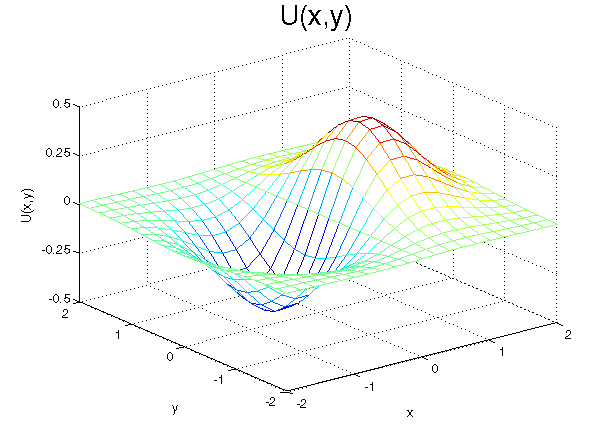
To understand Lagrangian Mechanics, we must abandon our idea of “force” as the fundamental phenomenon. Instead of forces, we deal with “potential fields”.

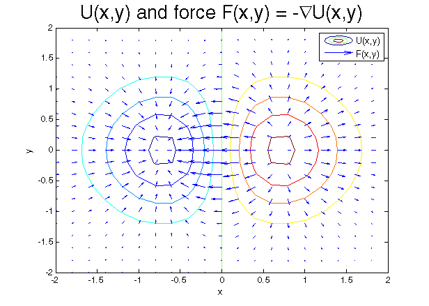
You can imagine potential fields as a roller coaster track, or as a landscape of rolling grassy hills. The height of a track or a landscape at that point corresponds to the value of the potential at that point. Potential fields work like this: Every object “wants” to go downwards in a potential field — it will want to go in the direction (backwards/forwards for the roller coaster, north/south/east/west for the hilly landscape) that will take it downwards. We don’t care why, or how — it just “wants” to. And the steeper the downwardness, the greater the compulsion.

We call this potential field \(U(\vec{r})\), which means “\(U\) at the point \(\vec{r}\)”. (\(\vec{r}\) denotes a point in space)

Relating this to \(F = m a\), the force on the object is now equal to the steepness of the potential field at the point where the object is, and in the direction that would allow the object to go downwards in potential. Objects always wish to minimize their potential, and do so as fast as they can. In mathematical terminology, we say that \(F(\vec{r}) = - \vec{\nabla} U(\vec{r})\).

Now, for Lagrangian Mechanics:

Let’s say I tell you an object’s location at time \(t_0\), and its location later at time \(t_1\), and the potential energy field. What path did that object take to get from point A to point B?

A pretty open question, right? You don’t really have that much information to go off of. You just know point A and point B. It could have taken any path, for all we know! If we only knew \(F = m a\), not only would we be at a complete loss at how to even start, but we wouldn’t even know if there was only one or even a hundred valid paths a particle could have taken.

The solution to this problem is actually rather unexpected. Consider every single path/curve from point A to point B. Every single one. Now, assign each path a number known as the Action:

1. For every point, add up the “Kinetic Energy” at that point, which, for classical mechanics, is the square of the object’s speed multiplied by \(\frac{1}{2} m\).
2. For every point, add up \(U(\vec{r})\) at that point.
3. Subtract (2) from (1).

Think about every possible path. Calculate the action for each one. The path that the object takes is the path with the lowest action

It’s almost as if the object “does the math” in its head: “I’m going to go from here to there…let me calculate which path I can take has the lowest action. Okay, got it!”

Lagrangian Mechanics provides for us a way to find out just what path an object must have taken to get from point A to point B.

As it turns out, looking at things this way opens up entire worlds of understanding. For example, just from this, we find that total energy is conserved over time for a closed system (trust me on this; the calculus is slightly tricky). We also have a formulation that works fine under Special Relativity in all frames of reference with almost no tweaks. And yes, if you actually do find the path of lowest action, the path will somehow magically always follow the state-updating equations \(F = m a\). It’s just now we have a much more insightful and meaningful way to look at the universe:

Paths always attempt to minimize their action.

Okay. We don’t have that much time to spend on this, or its philosophical implications, so we’re going to move on now to Quantum Mechanics.

Quantum Mechanics

Schrödinger Formulation

If there was one thing that “everyone” knew about quantum mechanics, it would either be Scrödinger’s Cat or the fact that objects are no longer “for sure” anywhere. They are only probably somewhere.

How can we then analyze the behavior of anything? If everything is just a probability, and nothing is certain, we can’t really use the same “state-updating functions” that we used to rely on, because the positions and velocities of the objects in question don’t even have well-defined values.

Physicists’ first solutions involved creating a new “state” that did not involve particles at all. This “state” described the state of the universe, but not in terms of particles and positions and velocities. It is a new abstract state. Then, they invented the equivalent of an \(F = m a\) for this abstract state — an equation that, for every abstract state at time \(t_0\), gives you the abstract state at time \(t_0 + \Delta t\).

This approach is useful…just like \(F = m a\) was useful. But it inherits all of the problems of \(F = m a\). How can we apply what we learned about actions and Lagrangian mechanics to Quantum Mechanics? How do we make Lagrangian mechanics “quantum”?

Path Integral Formulation

The answer is a bit simple, actually.

Instead of saying “the object will chose the path with the least action”, we say the object chooses a random path, choosing lower-action paths more often. That is, if an electron is shot from point A to point B, the electron picks a random path from point A to point B. It is a weighted random choice based on the action of each path — if Path \(\alpha\) has lower action than Path \(\beta\), the electron will pick path \(\alpha\) more often than path \(\beta\).

There are some small technical differences (the process of calculating the action is slightly different, and you end up summing over complex numbers for certain reasons), but the fundamental principle remains the same.

So say we have an electron floating around a hydrogen atom (a hydrogen atom creates a very pretty and easy to work with potential field). We know it is at point A at time \(t_0\), and point B at time \(t_1\). What path did the electron take to get there?

Simple: We don’t know. But we can say that it probably took the path with the least action. It could have also taken the path with the second to least action…but that’s just slightly less likely. It probably did not take the path with the greatest action…but who knows — it might have! It’s like it rolls a dice to determine which path it goes on, but the dice is weighted so that lower-action paths are rolled more often than higher-action paths.

The electron wants to take the lowest-action path…but sometimes decides not to.

So now we see what Lagrangian Mechanics in classical mechanics really is: It’s quantum mechanics, except that the lowest-action path is so much likelier than any other path that we almost never see the second-to-least action path taken.

As it turns out, like Lagrangian mechanics opened eyes to new worlds in classical mechanics, the Path Integral formulation¹ of quantum mechanics opened up totally new worlds that the previous “state updating formula” approach could have never dreamed of.

Implications

Okay, so what does this all have to do with us?

How many processes do we know that can be modeled by something trying to minimize itself, but not always succeeding? What data patterns can be unveiled by modeling things this way?

I’ll leave this question slightly open-ended, but I’m also going to hint at the next installment’s contents.

Particle in a potential

Let’s go back again to our electron next to an atom. Let’s say that this electron will move around and return back to its current position at time \(t_0 + \Delta t\), for very large \(\Delta t\). From what we learned, this electron can really take any path it wants, going anywhere in the universe and back again. Any closed loop that that zig zags or curls anywhere is a valid path.

We can “pick” a random path, weighted by the action, and see where the electron goes in that path. See where we find the electron along points in the path. After many picks, we start seeing where the electron is “most likely to be”. We find the probability distribution of an electron in that potential.

We now have a way, given any quantum potential, to find the probability distribution of a particle in that potential.

From here we can also find the particle’s average energy, and many other properties of a particle given an arbitrary quantum potential.

Now let’s implement it.

---

1. Why is it called the “Path Integral” formulation? When we add up something at every single point on a path, we are mathematically performing a “Path Integral”. So Path Integral Formulation means “physics based on the adding up stuff for every point on a path”.↩︎